Skip to content
 PENGUINS DATASET
 Multiclass Classification
Project
Field
Data Science
Stakeholders
Researchers, ecologists, and conservationists
S. Learning Project
Penguins Dataset
Description
The overarching goal of this project is to implement and demonstrate the understanding of concepts from supervised learning to a problem and dataset that resonates with you.
The project working should clearly explain the choice of analyses you make. The project should, at the end of the day, also serve as a comparative analysis of different machine learning models applied on the same dataset.
Its is expected that atleast three classical ML approaches and atleast neural network architecture will be implemented.
Comprehensive Index for a Multiclass Classification Project
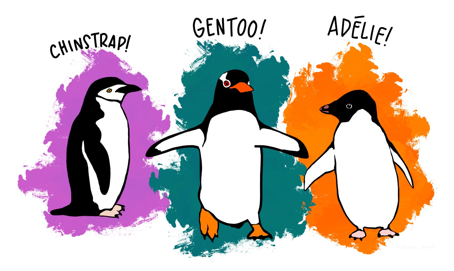
Introduction to the Penguins Project
Welcome to this insightful journey through the Penguins Project! The aim of this blog is to provide a comprehensive overview of the various steps undertaken in this fascinating project.
By the end, you’ll have a clear understanding of the techniques employed, allowing you to delve into the Jupyter notebook on GitHub to explore preprocessing, exploratory data analysis (EDA), and modeling sections.
All datasets, visualizations, and other generated insights are neatly organized in our GitHub Folder. For a deeper understanding of code navigation, consult the “README” file on GitHub, with the URL conveniently provided at the blog’s end.
Project Overview
The primary goal of this project is to construct a robust statistical learning model for multiclass classification of penguins based on key morphological features. The intentionally complex dataset incorporates challenges such as NA values and outliers, mirroring real-world scenarios.
The project culminates in a thorough model comparison, evaluating performance metrics to understand the impact of hyperparameters, feature selection, and overfitting mitigation across various models.
We’re committed to optimizing model training, exploring 14 distinct models, each with a unique approach. For every strategy, we deployed two models—one using all features and another focusing on essentials. Our exploration included LgR with Grid Search, SVM, Decision Trees, KNN, Naive Bayes, and NN.
Data Preprocessing
Dividing the Dataset
We initiated the project by dividing the dataset into training and validation sets, a crucial step to prevent data leakage.
Exploratory Data Analysis (EDA)
The EDA phase aimed to unveil patterns in the data. Handling missing values and outliers in separate datasets allowed us to glean more precise insights into our clean data.
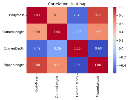
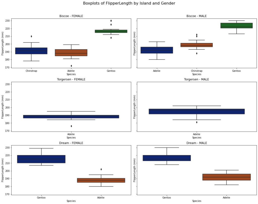
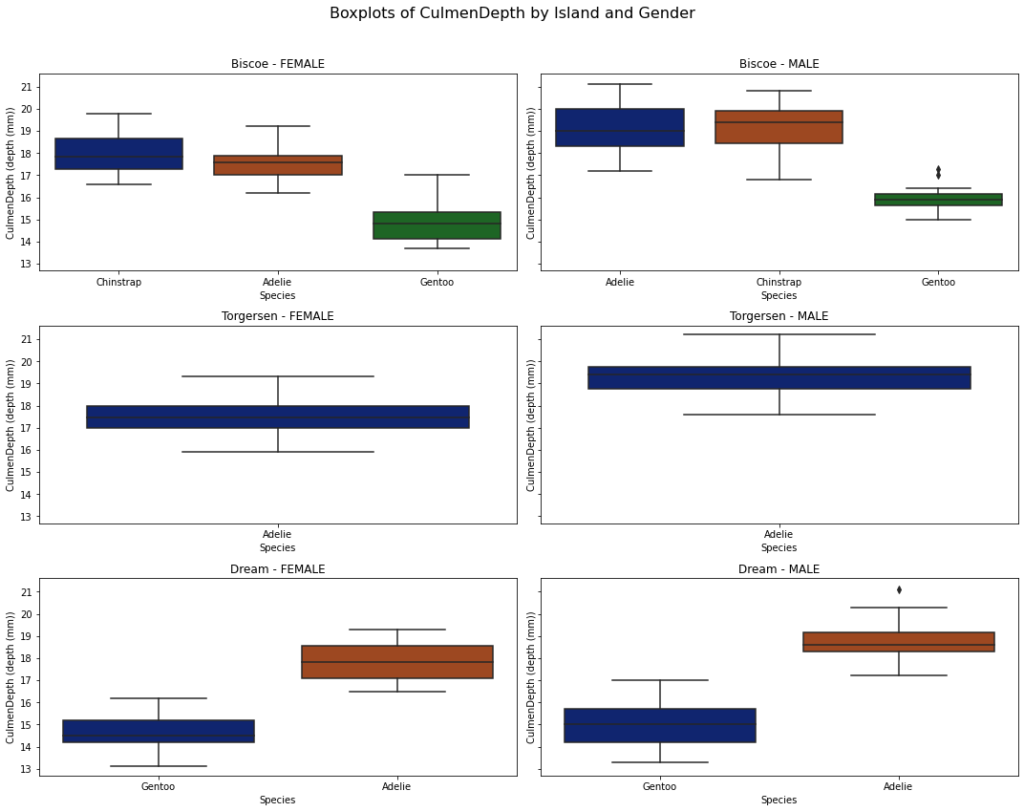
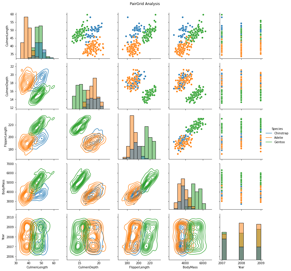
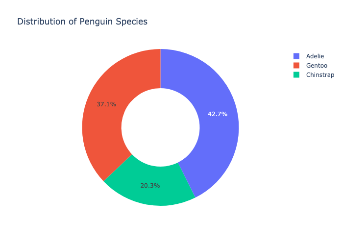
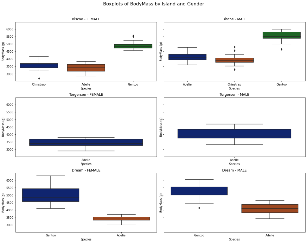
Visualizations, including pivoted tables, circle graphs, boxplots, scatterplots, and correlation maps, provided a profound understanding of penguin distribution, species attributes by sex, and attributes by island.
Correlated variables were identified and reserved for treatment in the modeling section. Prominent distinctions surfaced when analyzing different genders within species across various islands.
Outliers were imputed using the Interquartile Range (IQR) method, and missing values were addressed using SimpleImputer with mean imputation, considering specific combinations of species, island, and gender.
Normalization of non-normally distributed variables was accomplished using standardScaler(). Both numerical and categorical data were handled through encoding with Ordinal Encoder for ordinal features and LabelEncoder for binary features.
To address dataset imbalance, the Synthetic Minority Over-sampling Technique (SMOTE) was employed, generating synthetic samples for the minority class while preserving essential information from the majority class.
More Details
In the following section, I will showcase a curated selection of visualizations crafted in the Python document. To delve deeper into these visual insights, I encourage you to click on the “Project Notebook” button for a detailed exploration. Additionally, for a comprehensive view of the entire spectrum of visualizations, please click on the “All Visualizations” button.

Modeling
As showcased in the notebook, our commitment to optimizing model training led us to explore diverse approaches. We implemented 14 distinct models, each representing a unique strategy.
For each approach, we deployed two models: one utilizing all features and another focusing solely on the most crucial ones.
Our methodology encompassed LgR with Grid Search, SVM, Decision Trees, KNN, Naive Bayes, and NN, providing a comprehensive exploration of model architecture.
Hyperparameter Tuning
A grid of hyperparameters was defined for tuning, and grid search with cross-validation was performed to identify the best hyperparameter combination for training data across different models.
Model Comparison
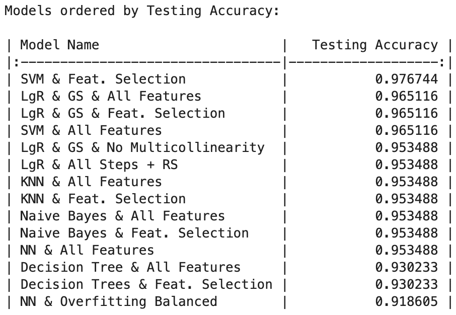
- Testing Accuracy:
SVM with Feature Selection achieved the highest testing accuracy at 97.67%, followed closely by Logistic Regression models with Grid Search (both All Features and Feature Selection) and SVM with All Features, all reaching 96.51%. KNN and Naive Bayes models (with and without Feature Selection) demonstrated commendable accuracy at 95.35%.
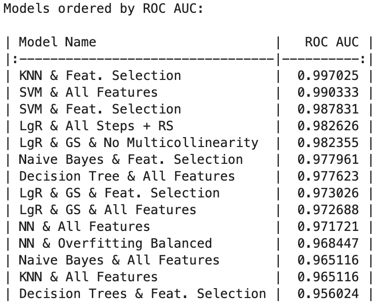
- ROC AUC:
KNN with Feature Selection led with an impressive ROC AUC of 99.70%, followed closely by SVM, which achieved 99.03% with all features and 98.78% with feature selection. Additionally, Logistic Regression with All Steps + Random Search and Logistic Regression with Grid Search and No Multicollinearity both surpassed 98.23%.
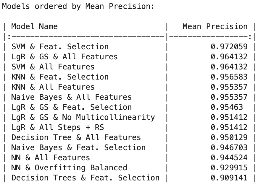
- Precision, Recall, and F1-Score:
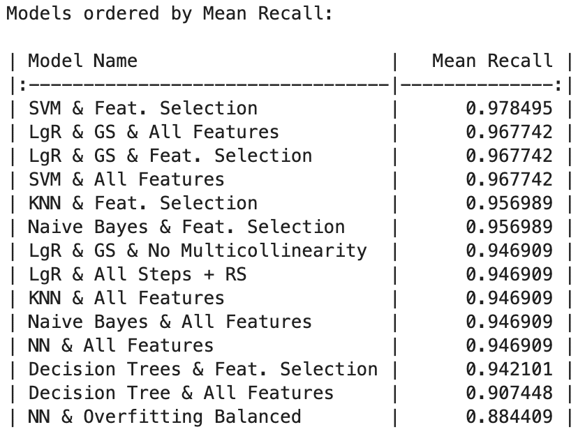
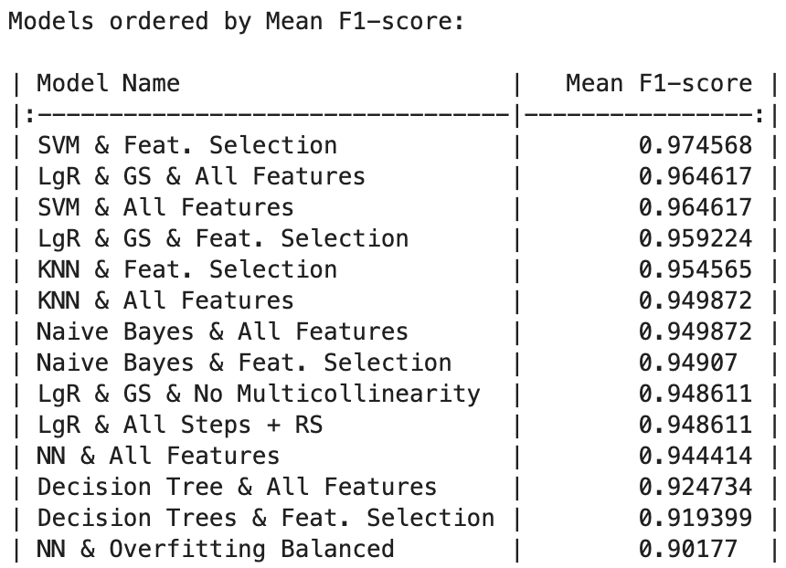
SVM stands out as the top-performing model across metrics, boasting exceptional precision (97.20%), recall (97.84%), and F1-score (97.45%). Following closely is Logistic Regression with Grid Search using All Features, excelling in precision (96.41%), recall (96.77%), and F1-score (96.46%). This underscores its ability to make accurate positive predictions while capturing a substantial portion of actual positive instances.
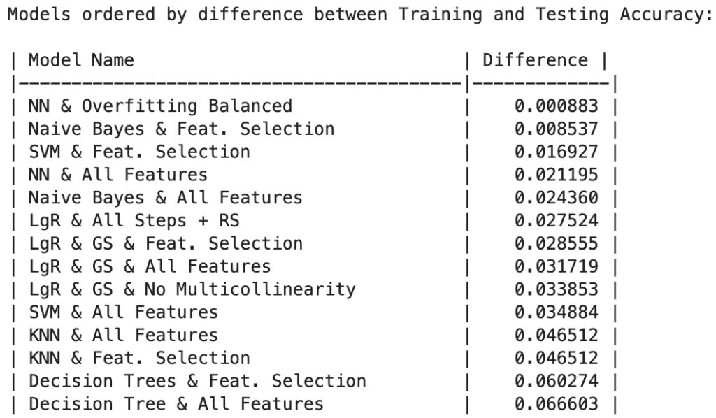
- Generalization and Overfitting:
Neural Network with Overfitting Balanced showcases minimal difference between training and testing accuracy (0.0008), emphasizing effective overfitting avoidance and consistent performance on unseen data. Notably, Naive Bayes models with Feature Selection, Neural Networks with All Features, and Naive Bayes and SVM with Feature Selection using All Features also demonstrate robustness, with differences of 0.0085 and 0.0169, respectively.
More Details
Below, you will discover visualizations organized by metrics. If you desire a more comprehensive view, including AUC values, ROC curves, confusion matrices, classification reports, and additional metrics, please click on the “Evaluation Metrics” button.
For an in-depth understanding of each model, presented in a step-by-step fashion, we strongly recommend clicking on the “Project Notebook” button.
Final Model Recommendation
Upon rigorous evaluation, Decision Tree models were excluded from consideration due to consistently inferior performance.
Although KNN and Logistic Regression models exhibited commendable metrics, they were set aside due to a notable disparity between testing and training accuracy, signaling potential overfitting.
Neural Network models faced elimination due to performance divergence and suboptimal metrics.
Exploring the utilization of SVM with feature selection presents a noteworthy possibility.
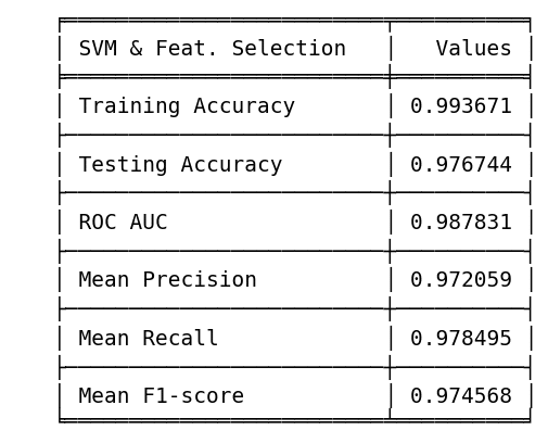
- Testing Accuracy: 1st position (0.9767).
- ROC AUC: 3rd position (0.9878).
- Mean Precision: 1st position (0.9720).
- Mean Recall: 1st position (0.9784).
- F1 Score: 1st position (0.9745).
- Training & Testing Tradeoff: 3rd position (0.0169).
While the training accuracy stands at an impressive 99.36%, the model delivers compelling results, securing notable positions in various metrics:
On the other hand, another option we can also use is Naïve Bayes with feature selection.
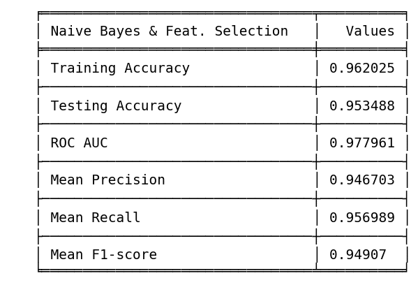
- Testing Accuracy: 6th position (0.9534)
- ROC AUC: 6th position (0.9779)
- Mean Precision: 11th position (0.9467)
- Mean Recall: 5th position (0.9569)
- F1 Score: 8th position (0.9490)
- Training & Testing Tradeoff: 2nd position (0.0085)
As observed, Naïve Bayes exhibits lower metrics compared to SVM; however, it demonstrates superior resilience against overfitting. This is evident in the minimal difference between our training and testing accuracy, all while maintaining commendable results.
By continuously tracking and evaluating their outputs, we can tailor our strategy to maximize the benefits derived from Naïve Bayes’ robustness against overfitting and SVM’s superior metric performance. This adaptive approach ensures a nuanced utilization of both models for optimal outcomes in diverse scenarios.
Improvement Analysis
Upon comprehensive review of the entire codebase, I’ve identified several areas where enhancements could significantly contribute to achieving superior results for our model. Let’s delve into these suggestions:
1. Data Split for Model Training: Given the relatively modest size of our dataset, optimizing the data split strategy becomes pivotal. Instead of the conventional 75/25 split, I propose adopting an 80/10/10 split for training, validation, and testing, respectively. This adjustment ensures a more robust training set while still allocating sufficient data for validation and testing:
- Training: 80% of the Total Dataset
- Validation: 10% of the Total Dataset
- Test: 10% of the Total Dataset
This modification provides a balanced approach, enhancing the model’s capacity to generalize effectively.
2. Improved Encoding Practices: A crucial aspect that requires attention is our encoding strategy. While some variables, like ‘year’ and the target variable, may be appropriately treated as ordinal, ‘island’ appears to be a nominal category. I recommend utilizing the One-Hot Encoder for the ‘island’ variable to accurately represent its categorical nature. This adjustment can significantly enhance the model’s understanding of this feature.
3. Fine-Tuning Hyperparameters: Throughout our hyperparameter tuning process, it became evident that certain parameters consistently hovered near the upper or lower bounds of our grid search thresholds. Although we opted not to redefine these hyperparameters to maintain project efficiency, a potential avenue for improvement is expanding the parameter range. By extending the search space for these critical hyperparameters, we may unlock additional performance gains and refine the model further.
4. Hyperparameters vs our Loss function: This analysis will help us identify the optimal balance between training and testing accuracy. This approach mirrors the successful strategy employed in our previous Neural Network model, where we continuously compared our Loss Function across epochs, effectively mitigating overfitting issues.
While these recommendations are not currently implemented in the existing codebase, they serve as valuable insights for potential improvements. As the primary focus shifts towards new data projects, the opportunity to implement these enhancements remains open. Should you wish to explore and practice with these suggestions to refine the model, feel free to incorporate them at your discretion.
Collectively, these proposed changes aim to elevate the model’s performance and contribute to a more accurate and robust outcome. If you decide to integrate these suggestions into your work, it could serve as an excellent exercise in refining the model’s capabilities!
In-Depth Report
Project Author Details